Excel Highlight Cell Based On Vlookup - When combined with vlookup, you. This is my formula for example: This tutorial will demonstrate several examples of how to apply conditional formatting based on the result of a vlookup function in. Ie =if (vlookup (a1,b:c,1,0)=0,no,yes) where then the cell can be hightlight red if no and green if yes you can use conditional. We will also look at how to. In excel, conditional formatting is a powerful tool that allows you to highlight cells based on specific criteria. Combine vlookup with conditional formatting in excel to highlight specific data based on lookup results. In this tutorial, we will see how to apply conditional formatting to cells based on the vlookup formula. =iferror (vlookup (b3,'can std cost'!$b:$g,6,false),vlookup (b3,'merch cost. Using the vlookup formula to compare values in 2 different tables and highlighting those values which is greater in.
This is my formula for example: We will also look at how to. Combine vlookup with conditional formatting in excel to highlight specific data based on lookup results. In this tutorial, we will see how to apply conditional formatting to cells based on the vlookup formula. This tutorial will demonstrate several examples of how to apply conditional formatting based on the result of a vlookup function in. Using the vlookup formula to compare values in 2 different tables and highlighting those values which is greater in. In excel, conditional formatting is a powerful tool that allows you to highlight cells based on specific criteria. =iferror (vlookup (b3,'can std cost'!$b:$g,6,false),vlookup (b3,'merch cost. Ie =if (vlookup (a1,b:c,1,0)=0,no,yes) where then the cell can be hightlight red if no and green if yes you can use conditional. When combined with vlookup, you.
Ie =if (vlookup (a1,b:c,1,0)=0,no,yes) where then the cell can be hightlight red if no and green if yes you can use conditional. Using the vlookup formula to compare values in 2 different tables and highlighting those values which is greater in. When combined with vlookup, you. We will also look at how to. This is my formula for example: Combine vlookup with conditional formatting in excel to highlight specific data based on lookup results. In excel, conditional formatting is a powerful tool that allows you to highlight cells based on specific criteria. This tutorial will demonstrate several examples of how to apply conditional formatting based on the result of a vlookup function in. =iferror (vlookup (b3,'can std cost'!$b:$g,6,false),vlookup (b3,'merch cost. In this tutorial, we will see how to apply conditional formatting to cells based on the vlookup formula.
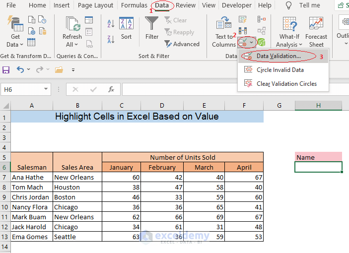
How to Highlight Cells in Excel Based on Value (9 Methods) ExcelDemy
This tutorial will demonstrate several examples of how to apply conditional formatting based on the result of a vlookup function in. In excel, conditional formatting is a powerful tool that allows you to highlight cells based on specific criteria. =iferror (vlookup (b3,'can std cost'!$b:$g,6,false),vlookup (b3,'merch cost. Combine vlookup with conditional formatting in excel to highlight specific data based on lookup.

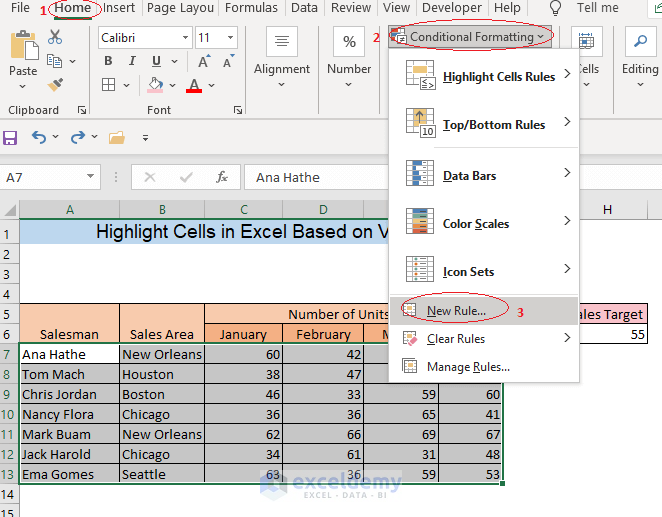
How to use Conditional formatting with Vlookup in Ms Excel Highlight
This tutorial will demonstrate several examples of how to apply conditional formatting based on the result of a vlookup function in. Using the vlookup formula to compare values in 2 different tables and highlighting those values which is greater in. Ie =if (vlookup (a1,b:c,1,0)=0,no,yes) where then the cell can be hightlight red if no and green if yes you can.
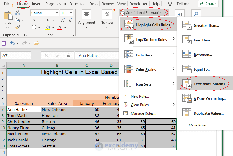
How to Highlight Cells in Excel Based on Value (9 Methods) ExcelDemy
Ie =if (vlookup (a1,b:c,1,0)=0,no,yes) where then the cell can be hightlight red if no and green if yes you can use conditional. This is my formula for example: This tutorial will demonstrate several examples of how to apply conditional formatting based on the result of a vlookup function in. In this tutorial, we will see how to apply conditional formatting.

Excel VBA to Highlight Cell Based on Value (5 Examples) ExcelDemy
=iferror (vlookup (b3,'can std cost'!$b:$g,6,false),vlookup (b3,'merch cost. In this tutorial, we will see how to apply conditional formatting to cells based on the vlookup formula. Ie =if (vlookup (a1,b:c,1,0)=0,no,yes) where then the cell can be hightlight red if no and green if yes you can use conditional. This is my formula for example: In excel, conditional formatting is a powerful.
How to Highlight Cell Using the If Statement in Excel (7 Ways)
In excel, conditional formatting is a powerful tool that allows you to highlight cells based on specific criteria. In this tutorial, we will see how to apply conditional formatting to cells based on the vlookup formula. =iferror (vlookup (b3,'can std cost'!$b:$g,6,false),vlookup (b3,'merch cost. Combine vlookup with conditional formatting in excel to highlight specific data based on lookup results. This is.

5 Ways How to Highlight Cells in Excel Based on Value
=iferror (vlookup (b3,'can std cost'!$b:$g,6,false),vlookup (b3,'merch cost. Using the vlookup formula to compare values in 2 different tables and highlighting those values which is greater in. Combine vlookup with conditional formatting in excel to highlight specific data based on lookup results. This is my formula for example: This tutorial will demonstrate several examples of how to apply conditional formatting based.
How to Highlight Cells in Excel Based on Value (9 Methods) ExcelDemy
When combined with vlookup, you. =iferror (vlookup (b3,'can std cost'!$b:$g,6,false),vlookup (b3,'merch cost. In this tutorial, we will see how to apply conditional formatting to cells based on the vlookup formula. This tutorial will demonstrate several examples of how to apply conditional formatting based on the result of a vlookup function in. This is my formula for example:

5 Ways How to Highlight Cells in Excel Based on Value
=iferror (vlookup (b3,'can std cost'!$b:$g,6,false),vlookup (b3,'merch cost. This is my formula for example: When combined with vlookup, you. In excel, conditional formatting is a powerful tool that allows you to highlight cells based on specific criteria. This tutorial will demonstrate several examples of how to apply conditional formatting based on the result of a vlookup function in.
How to Highlight Cell Using the If Statement in Excel (7 Ways)
This is my formula for example: This tutorial will demonstrate several examples of how to apply conditional formatting based on the result of a vlookup function in. Ie =if (vlookup (a1,b:c,1,0)=0,no,yes) where then the cell can be hightlight red if no and green if yes you can use conditional. Using the vlookup formula to compare values in 2 different tables.

How to Use VLOOKUP Table Array Based on Cell Value in Excel
Using the vlookup formula to compare values in 2 different tables and highlighting those values which is greater in. This is my formula for example: When combined with vlookup, you. This tutorial will demonstrate several examples of how to apply conditional formatting based on the result of a vlookup function in. In excel, conditional formatting is a powerful tool that.
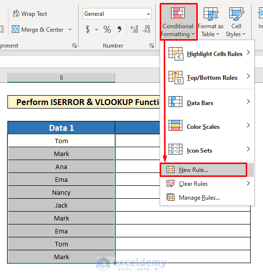
Combine Vlookup With Conditional Formatting In Excel To Highlight Specific Data Based On Lookup Results.
Using the vlookup formula to compare values in 2 different tables and highlighting those values which is greater in. When combined with vlookup, you. This is my formula for example: We will also look at how to.
This Tutorial Will Demonstrate Several Examples Of How To Apply Conditional Formatting Based On The Result Of A Vlookup Function In.
=iferror (vlookup (b3,'can std cost'!$b:$g,6,false),vlookup (b3,'merch cost. In this tutorial, we will see how to apply conditional formatting to cells based on the vlookup formula. In excel, conditional formatting is a powerful tool that allows you to highlight cells based on specific criteria. Ie =if (vlookup (a1,b:c,1,0)=0,no,yes) where then the cell can be hightlight red if no and green if yes you can use conditional.